Frequency domain
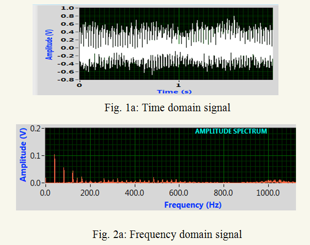
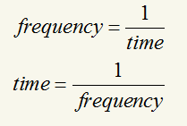
In cases of measuring the level of distortion in an audio oscillator or detection of the first sounds of a bearing failing on noisy machine, we are trying to detect a small sine wave in the presence of large signals. Fig. 1a shows a time domain signal of bearing measure data which seems non-periodic signals. But Fig. 1b shows the frequency domain that the same signal is composed of a large sine wave and other sine wave components. When these components are separated in frequency domain, the smaller components can be easily detected. The frequency domain's usefulness is not restricted to electronics or mechanics. This is a useful tool in analyzing important effects of large signal in time domain almost in all fields of engineering and science.
Frequency spectrum
Frequency spectrum is representation of time-domain signal in frequency domain. This can be generated by applying Fourier transform to signal, which can be represented in amplitude versus frequency as shown in Fig. 2. In simply, the time domain graph is called the waveform, and the frequency domain graph is called the spectrum. It is easy to analyse physical discretion of their internal process in frequency spectrum for the real phenomena. Often, the frequency spectrum clearly shows harmonics, visible as lines, which provides insight into the mechanisms that generate the entire signal. Relation between time and frequency as follows
Spectrum analysis is technical process of decomposition of the complex waves into simpler parts. By this analysis, we can quantify the various amounts such as amplitude, powers, intensities or phases. This analysis can be performing on entire signal or the sort segment (sometimes called frames) of a signal. The obtained information is key for understanding the mechanism of signal. The Fourier transform is used to extract this information.
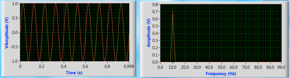
Fig 2a: Sine waveform in time ang frequency domains
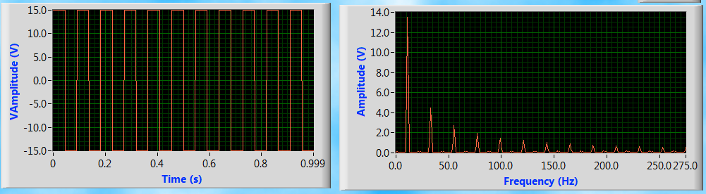
Fig 2a: Sine waveform in time ang frequency domains
Fig. 2 shows a few common signals in time and frequency domains. The spectrum of sine signal is a single line. From Fig. 2b, the square wave is composed of an infinite number of sine waves, are harmonically related. The lowest frequency present is the reciprocal of the square wave period. From above two examples, one can judge that a signal which is a periodic and exists for all time has a discrete frequency spectrum. For the transient signal, the frequency spectrum is continuous. This means that the sine waves which make this signal are spaced infinitesimally close together. In case of impulse signals, the frequency spectrum is flat i.e. there is energy at all frequencies.
Types of Fourier transforms
Fourier series
Transforms an infinite periodic time signal into an infinite discrete frequency spectrum
Fourier Integral Transform
Transforms an infinite continuous time signal into an infinite continuous frequency spectrum
Discrete Fourier Transform (DFT)
Transforms a discrete periodic time signal into a discrete periodic frequency spectrum
Fast Fourier Transform
A computer algorithm for calculating the DFT
Digital Fourier analysis
The Discrete and Fast Fourier transform algorithms are the tools for quick and easy application of Fourier theory. The Discrete and Fast Fourier transform operates on finite sequences-sets of data with each point discretely and evenly spaced in time. However,, the waveforms usually in analog nature which are in continuous in time, and they must be sampled at discrete points before the DFT and FFT algorithms can be applied. And, to be processed by a digital computer, these sampled points must be digitized as well. Understanding two basic concepts of the full analog-to-digital conversion, namely windowing and sampling, will put a long way down the road to appreciating the FFT and understanding its results.
Aliasing
It is important that there is no information in the sampled waveform near the sampling frequency to avoid a problem called aliasing.
Now note what happens if the actual signal is higher in frequency than the sampling frequency. The sampler output looks like a very low frequency, and again it is not a correct representation of the actual signal. This phenomenon is called aliasing, and it can lead to gross errors unless it is avoided. The best way to avoid aliasing is to pass the input signal through an analog low-pass filter whose cut-off frequency is less than one-half the sampling frequency.
Sampling Rules for Digital Signal Analysis
The data path must contain an analog Anti-Aliasing low-pass filter
You must sample at least twice as fast as the highest frequency to be analyzed
The Frequency Response of the analysis depends on the sampling frequency
These rules apply to all FFT analysis, and the analyzer automatically takes care of them. The anti-aliasing filter is internally set to the appropriate value for each frequency range of the analyzer. The total sampling time is called the time record length and the nature of the FFT dictates that the spacing between the frequency components in the spectrum (also called the frequency resolution) is 1 divided by the record length. For instance, if the frequency resolution is one Hz, then the record length is one second, and if the resolution is 0.1 Hz, then the record length is 10 seconds, etc. From this it can be seen that in order to perform high resolution spectrum analysis relatively long times are required to collect the data. This has nothing to do with the speed of the calculations in the analyzer; it is simply a natural law of frequency analysis.
Leakage
The FFT analyzer is a batch processing device; that is it samples the input signal for a specific time interval collecting the samples in a buffer, after which it performs the FFT calculation on that "batch" and displays the resulting spectrum.
If a sinusoidal signal waveform is passing through zero level at the beginning and end of the time record, i.e., if the time record encompasses exactly an integral number of cycles of the waveform, the resulting FFT spectrum will consist of a single line with the correct amplitude and at the correct frequency. If, on the other hand, the signal level is not at zero at one or both ends of the time record, truncation of the waveform will occur, resulting in a discontinuity in the sampled signal. This discontinuity is not handled well by the FFT process, and the result is a smearing of the spectrum from a single line into adjacent lines. This is called "leakage"; it is as if the energy in the signal "leaks" from its proper location into the adjacent lines.
Windowing
In order to reduce the effect of leakage, it is necessary to see to it that the signal level is zero at the beginning and end of the time record. Multiplying the data samples by a so-called "windowing" or "weighting" function, this can have several different shapes, does this. The most common forms of windows and their uses are considered next.
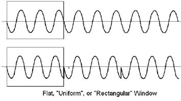
If there is no windowing function used, this is called "Rectangular", "Flat", or "Uniform" windowing. In the figure above, the effect of the data truncation can be seen as discontinuities in the windowed waveform. The FFT analyzer only knows what is in the time window, or time record. It assumes the actual signal contains the discontinuities, and they are the cause of the leakage seen in the previous figure. Leakage could be avoided if the input waveform zero crossings were synchronized with the sampling times, but this is impossible to achieve in practice.
For detailed description of different types of windows can be obtained from articles which are attached in references section.
Ageraging
One of the important functions of the FFT analyzer is that it is easily able to do averaging of spectra over time. In general, the vibration signal from a rotating machine is not completely deterministic, but has some random noise superimposed on it. Because the noise is unpredictable, it alters the spectrum shape, and in many cases can seriously distort the spectrum. If a series of spectra are averaged together, the noise will gradually assume a smooth shape, and the spectral peaks due to the deterministic part of the signal will stand out and their levels will be more accurately represented. It is not true that simply averaging FFT spectra will reduce the amount of the noise -- the noise will be smoothed but its level will not be reduced.
There are two types of averaging in general use in FFT analyzers, called linear averaging and exponential averaging. Linear averaging is the adding together of a number of spectra and then dividing the total by the number that was added. This is done for each line of the spectra and the result is a true arithmetic average on a line-by-line basis. Exponential averaging generates a continuous running average where the most recently collected spectra have more influence on the average than older ones. This provides a convenient form to examine changing data but still have the benefit of some averaging to smooth the spectra and reduce the apparent noisiness of them.
Time Synchronous Averaging
Time synchronous averaging, also called time domain averaging, is a completely different type of averaging, where the waveform itself is averaged in a buffer before the FFT is calculated. In order to do time domain averaging, a reference trigger pulse must be input to the analyzer to tell it when to start sampling the signal. This trigger is typically synchronized with an element of the machine that is of interest.
The average gradually accumulates those portions of the signal that are synchronized with the trigger, and other parts of the signal, such as noise, are effectively averaged out. This is the only type of averaging which actually does reduce noise.
source: http://www.dliengineering.com/vibman/averaging.htm