Fault diagnosis
1.Balancing
1.1 Single Plane Balancing
To illustrate the principles of single – plane balancing, the motion of a symmetric rigid rotor is considered. The rotor is mounted on general anisotropic supports; that is, the support stiffnesses may be different in the x and y directions but, for illustration proposes, the angular degrees of freedom of the rotor are neglected so that the rotor may be modeled using only two translational degrees of freedom. In effect, we are assuming that any unbalance present lies on a plane of symmetry normal to the axis of the rotor and that the stiffness’s of the supports on either side of this plane are identical. Unbalanced corrections also are applied at this plane.
Suppose that the initial response of the rotor, at spin speed Ω, is r0. If an additional unbalance bc (=mcƐc) is fixed to the balancing plane, a new response, rc, is measured after the rotor is accelerated to the same speed, Ω. Assuming that the rotor system behaves linearly, this new response can be written as
![]()
Where R (Ω)is a response function of the trial balance added. The objective is to determine the appropriate unbalance correction, bc, such that rc=0. Evidently, this requires knowledge of R (Ω). If a reliable numerical model is available, it may be used; however, this model must represent not only the mechanical dynamics of the rotor system but also a dynamics and gains of measurement system used. In practice, it is preferable to establish this response function by testing.
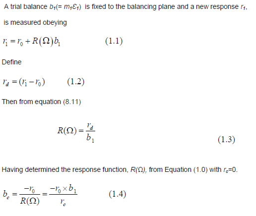
A practical issue is evident in equation (1.4). Calculating the corrective unbalance involves a division by the quantity rd. if this quantity is small in magnitude compared to the magnitude of r0. Then the degree of uncertainty on this number due to noise, sensor errors, quantization errors, or numerical rounding may be significant. It is standard practice to select b1 such that |rd| is similar to |r0|.