Theoretical Analysis
Finite element formulation of Rotor-Bearing Systems
The finite element model shown here is single disc rotor-bearing system .The stiffness and damping matrices mentioned can be used in rotor-bearing systems.
The system characteristic equation will be assembled considering individual components using finite element method (Nelson, 1980; Ozguven and Ozkan, 1984).
Finite rotor element
A two dimensional beam element shown in Figure 2 having four degrees of freedom per node is used for modelling the shaft.
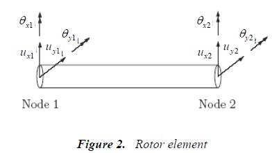
When the rotor is very thin, the effect of rotary inertia and shear deformation can be neglected. In other words Euler-Bernoulli beam theory is accurate enough as compared to the Timoshenko beam theory which considers the rotations due to shear deformation and is therefore more appropriate for thick beams. A Timoshenko beam element with four degrees of freedom per node is considered for present analysis (Ozguven and Ozkan, 1984), whose equation of motion is given as
![]()
Baring Element
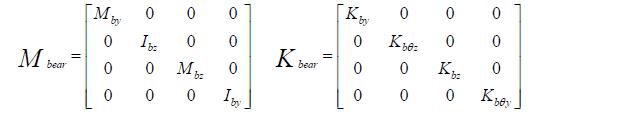
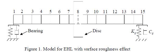
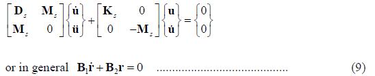
Most rotors are supported on oil-film bearings or in rolling contact bearings. The bearings The bearings influence the rotor vibrations to a certain degree by their dynamic properties. This influence originates essentially from the ratio of the rotor stiffness to the bearing stiffness. The bearings are modelled by stiffness and damping elements horizontal as well as in vertical plane as shown in Figure 1, where i,j = 1,2,....4 for four degrees of freedom. Neglecting the mass of bearing, the equation of motion for bearing can be written as,
![]()
where suffix ‘b’ corresponds to the bearing degrees of freedom, for example in Figure 1, suffix ‘b’ is referred to node numbers 1 and 15.
Rigid disc
The disc is assumed to have an effect like a concentrated mass and so it can be characterised solely by kinetic energies. Mass and inertia properties can be concentrated on the corresponding node on the shaft (Nelson and McVaugh, 1976). Hence, disc element with a single node and four degrees of freedom (as in Figure 1) has been used for modelling the disc.
![]()
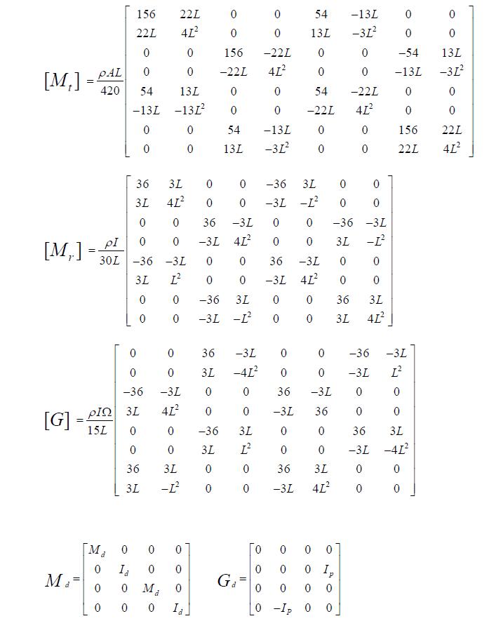
Where ![]() are the mass and gyroscopic matrices of the disc. Suffix ‘d’ corresponds to the disc nodal degrees of freedom, for example in Figure 1 suffix ‘d’ is referred to the node number 8.
are the mass and gyroscopic matrices of the disc. Suffix ‘d’ corresponds to the disc nodal degrees of freedom, for example in Figure 1 suffix ‘d’ is referred to the node number 8.
System equation of motion
After assembling equations (1-3), the system equation of motion becomes
![]()
where, ‘s’ stands for system,![]() is the global mass matrix of the system that includes the mass matrices of shaft and disc.
is the global mass matrix of the system that includes the mass matrices of shaft and disc.![]() matrix includes damping matrices of shaft and bearings as well as gyroscopic matrices of shaft and disc. The global stiffness matrix
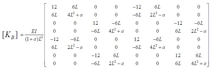
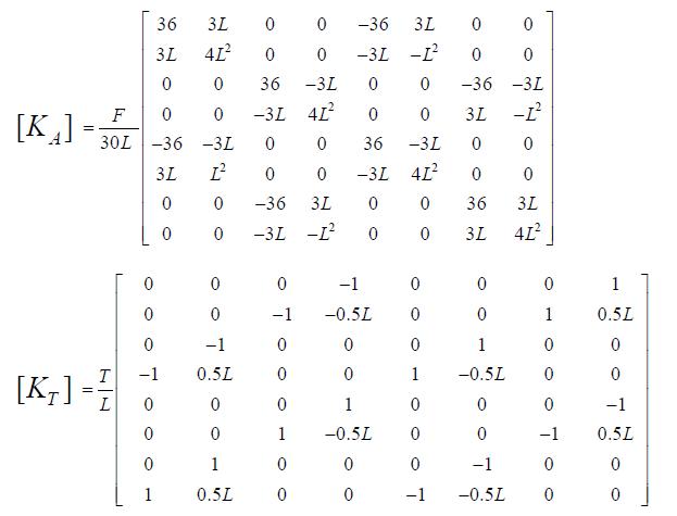
matrix includes damping matrices of shaft and bearings as well as gyroscopic matrices of shaft and disc. The global stiffness matrix![]() is the contribution of stiffness matrices of shaft and bearings. All the individual elemental matrices for beam element and disc are given in Appendix – E. The equation (4) can be solved using state-space method in the absence of external excitation for the Eigen analysis. The forced vibration characteristics can be studied with inclusion of external excitation force.
is the contribution of stiffness matrices of shaft and bearings. All the individual elemental matrices for beam element and disc are given in Appendix – E. The equation (4) can be solved using state-space method in the absence of external excitation for the Eigen analysis. The forced vibration characteristics can be studied with inclusion of external excitation force.
Eigen Value Problem
The eigenvalue problem becomes complex due to the inclusion of damping in the equation of motion. Such problems are not amenable to direct numerical applications as the computational costs involved would be higher than for the simple undamped case (Ewins, 2000). Therefore, the equations will normally be transformed into the State-Space form.
The equation of motion for free vibration is given by
![]()
Assuming a harmonic response, the rotor displacement can be represented by,
![]()
Substituting equation (6) into equation (5) leads to
![]()
which constitutes a complex eigenvalue problem. To transform the equation (7) into State-Space form, a new state vector is defined as

Finally from equations (5) and (8), the state space form is given as,
The formulation is often called the State-Space analysis, by contrast with usual vector-space analysis.![]() are 2Nx2N real symmetric matrices. The equation (9) is in a standard eigenvalue form which can be easily solved for 2N eigenvalues and eigenvectors. Assuming a solution form,
are 2Nx2N real symmetric matrices. The equation (9) is in a standard eigenvalue form which can be easily solved for 2N eigenvalues and eigenvectors. Assuming a solution form,![]() for the homogeneous case of equation (4), the associated eigenvalue problem is
for the homogeneous case of equation (4), the associated eigenvalue problem is
![]()
where,![]() The eigenvalues evaluated from equation (10) are in complex form,
The eigenvalues evaluated from equation (10) are in complex form, ![]() The imaginary part of the eigenvalue will give the system natural whirl frequency and real part will give about system damping. The logarithmic decrement defined as
The imaginary part of the eigenvalue will give the system natural whirl frequency and real part will give about system damping. The logarithmic decrement defined as ![]() indicates the stability threshold when
indicates the stability threshold when ![]()
Unbalance Response
Considering only the unbalance of disc, force for equation (4) can be of the form
![]()
A steady state solution of the same form,
![]()
is assumed and substituted in equation (4), which yields the solutions
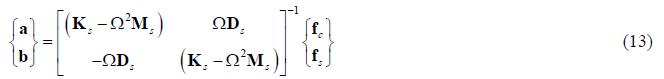
The back substitution of equation (13) into equations (12) provides system unbalance response.
All system matrices are represented conventional notations, can be found in Bettig (1996), Nelson and McVaugh (1976). Values of a, F and T are considered to be zero for the work presented in this thesis. However, it is possible to extend the work by considering these values non-zero, as the FEA code is developed including all the matrices mentioned in this appendix.